Analyzing the MOMA collection with pandas

New York’s Museum of Modern Art recently posted a CSV database of their collection on Github. It’s a great dataset to demonstrate some of the expressive power and user-friendly interface of pandas. That’s what this post is intended to do.

The dataset is also a chance to play with sexmachine, a python library that attempts to infer a person’s gender based on their name, which I’ll do in the next post.

%matplotlib inline
import matplotlib.pyplot as plt
import pandas as pd
import seaborn as sns
sns.set_context('poster')

Read and clean the data

pandas has a read_csv function that can read a CSV to the fundamental pandas object, the DataFrame. Each DataFrame has an index, which can be thought of a special column that identifies the rows. It can be generated automatically (e.g. as a sequence of integers beginning at zero), or you can tell read_csv to use a field of the source data, which we do below (the 12th column of the CSV is the unique MOMA ID of the item). We also tell read_csv to treat the 10th column as a datetime, which means it will parse the strings in that column into python datetimes.

# Use MOMA's ID as index
# Parse `DateAcquired` column as a datetime
moma = pd.read_csv('Artworks.csv', index_col=12, parse_dates=[10])

To sanity check the data, you can look at, e.g. moma.iloc[0] (the 0th record).

Title             Ferdinandsbrücke Project, Vienna, Austria , El...
Artist                                                   Otto Wagner
ArtistBio                                      (Austrian, 1841–1918)
Date                                                            1896
Medium                 Ink and cut-and-pasted painted pages on paper
Dimensions                        19 1/8 x 66 1/2" (48.6 x 168.9 cm)
CreditLine         Fractional and promised gift of Jo Carole and ...
MoMANumber                                                  885.1996
Classification                             A&D Architectural Drawing
Department                                     Architecture & Design
DateAcquired                                     1996-04-09 00:00:00
CuratorApproved                                                    Y
URL                           http://www.moma.org/collection/works/2
Name: 2, dtype: object

Note here that moma.loc[0] does not exist. loc addresses the index of the DataFrame, which in ours is the MOMA ID. The MOMA collection does not have an item with a MOMA ID of 0.

I then convert the categorical columns to pandas category dtypes.

categorical_columns = ['Classification', 'Department', 'CuratorApproved']

for c in categorical_columns:
    moma[c] = moma[c].astype('category')
    print(c, '\n', moma[c].cat.categories)

You can then inspect the categories:

Classification 
 Index(['(not assigned)', 'A&D Architectural Drawing',
       'A&D Architectural Model', 'A&D Design', 'A&D Graphic Design',
       'A&D Mies van der Rohe Archive', 'A&D Photograph', 'Audio', 'Collage',
       'Drawing', 'Film', 'Film (object)', 'Illustrated Book', 'Installation',
       'Media', 'Multiple', 'Painting', 'Performance', 'Periodical',
       'Photograph', 'Photography Research/Reference', 'Print', 'Sculpture',
       'Textile', 'Video', 'Work on Paper'],
      dtype='object')
Department 
 Index(['Architecture & Design', 'Architecture & Design - Image Archive',
       'Drawings', 'Film', 'Fluxus Collection', 'Media and Performance Art',
       'Painting & Sculpture', 'Photography', 'Prints & Illustrated Books'],
      dtype='object')
CuratorApproved 
 Index(['N', 'Y'], dtype='object')

Most of the plots below depend on the DateAcquired field being valid, so let’s use dropna to drop the 4428 records where this field is invalid or missing.

moma = moma.dropna(subset=['DateAcquired'])

Classifications and departments

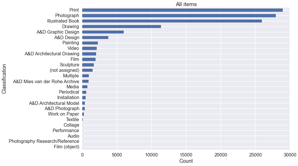
Having loaded the data, we can begin by examining the distribution of items in the collection by classification.

The chain of pandas operations required to do this has a lot going on in it, so let’s break it down:

• First we use a pandas groupby to group the moma DataFrame by Classification. This is analogous to a SQL GROUP BY operation. moma.groupby('Classification') is a DataFrameGroupBy object, which can be thought of as a list of pandas DataFrames each of which is made by splitting up the original DataFrame according to the value of Classification for each row.
• You can iterate over this list, but it’s usually more useful to perform an aggregation on it, i.e. to collapse each DataFrames the DataFrameGroupBy object into a single row. I just want to know how many items there are in each class, so I use .size().
• moma.groupby('Classification').size() is then a pandas Series, which we can sort and plot as a horizontal bar graph (kind='barh').

ax = (moma.groupby('Classification')
      .size()
      .sort_values()
      .plot(kind='barh'))

ax.set_title('All items')
ax.set_xlabel('Count');

We can do the same thing by Department.

ax = (moma.groupby('Department')
      .size()
      .sort_values()
      .plot(kind='barh'))

ax.set_title('All items')
ax.set_xlabel('Count');

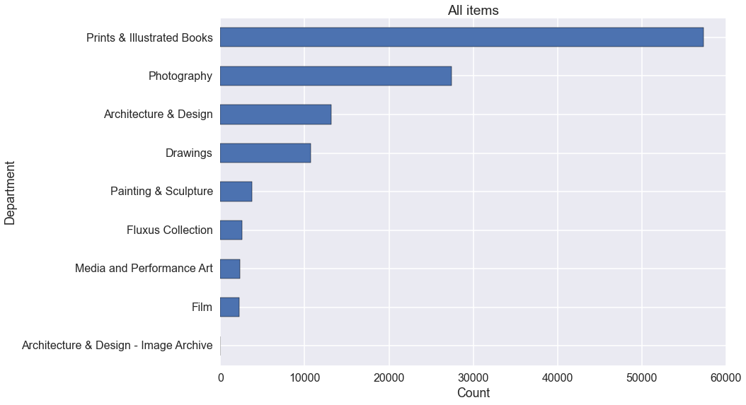
For obvious reasons, there are many more prints, photographs and books than any other class of work. If you’re only interested in paintings, sculptures and installations then records where Department is Paintings & Sculpture provides a way to select those out.

Artists

Which artists have the most items in the MOMA collection?

We can do this with the same groupby(), size() and sort_values() operations. The only difference here is that I add a tail() after the sort(), which gives us a list of the top 20 artists (sort_values() is ascending by default).

(moma.groupby('Artist')
 .size()
 .sort_values()
 .tail(20)
 .plot(kind='barh'))

ax.set_title('Artists with the most items in the MOMA collection (top 20)')
ax.set_xlabel('Count');

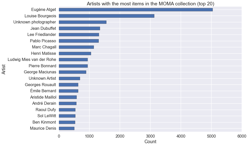
Lots of photographers! What if we only look at the Painting & Sculpture Department?

To do this, we need to filter the moma DataFrame before we operate on it. Inside the square brackets is moma['Department'] == 'Painting & Sculpture'. This is itself a Series, but its values are booleans (True and False. When this object is used to index a DataFrame (or Series), rows where the boolean Series is False are filtered out.

(moma[moma['Department'] == 'Painting & Sculpture']
 .groupby('Artist')
 .size()
 .sort_values()
 .tail(20)
 .plot(kind='barh'))

ax.set_title('Artists with the most items in the MOMA Painting & Sculpture department (top 20)')
ax.set_xlabel('Count');

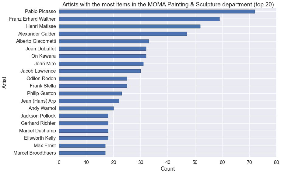
Lots of men! (I’ll revisit that in the next post.)

Overall trends with time

Looking at patterns with time (rather than by an unordered category like Department) is tricky, but easier in pandas than it would otherwise be!

We can give groubpy() a Grouper object to group into time intervals. The constructor for this object takes:

• a key keyword which tells the groupby operation which column contains the datetime we’re grouping by, and
• freq keyword, which is usually a string denoting some frequency. In this case, 'A' denotes year end. We could have used 'AS' for year start, or 'Q' for quarter end, or any of the other offset aliases defined by pandas.

Months of the year and days of the week are not intervals of time but rather recurring bins of time, so we don’t use the Grouper() objects for those. Rather, we use the .dt accessor to pull out the datetime object, and then the .month or .weekday to pick out the month or day of the week from DateAcquired field of the datetime object in that field. We can then groupby that. (And do some tedious work to fix the axes labels.)

fig, ax = plt.subplots(3, 1);
ylabel = 'Acquisitions'

(moma.groupby(pd.Grouper(freq='A', key='DateAcquired'))
 .size()
 .plot(ax=ax[0]))

(moma
 .groupby(moma['DateAcquired'].dt.month)
 .size()
 .plot(ax=ax[1]))

(moma.
 groupby(moma['DateAcquired'].dt.weekday)
 .size()
 .plot(ax=ax[2]))

months = {0: '_', 1: 'Jan', 2: 'Feb', 3: 'Mar', 4: 'Apr', 
        5: 'May', 6: 'Jun', 7: 'Jul', 8: 'Aug', 9: 'Sep', 
        10: 'Oct', 11: 'Nov', 12: 'Dec'}
days = {0: 'Mon', 1: 'Tue', 2: 'Wed', 3: 'Thu', 4: 'Fri', 5: 'Sat', 6: 'Sun'}

ax[0].set_title('MOMA acquisition trends with time')
ax[1].set_xticklabels([months[i] for i in ax[1].get_xticks()]);
ax[2].set_xticklabels([days[i] for i in ax[2].get_xticks()]);

for a in ax:
    a.set_xlabel('');
    a.set_ylabel(ylabel);

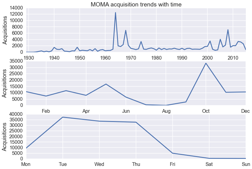
Lots of acquisitions in 1964, 1968 and 2008. More acquisitions in October than any other month. And Tuesdays are busy!

What happened in 1964? First let’s look at the year in detail using pandas datetime slicing, which allows you to use simple strings to refer to datetimes and construct a boolean Series with which to filter the DataFrame.

(moma[(moma['DateAcquired'] > '1964-01-01') &
      (moma['DateAcquired'] < '1964-12-31')]
 .groupby([pd.Grouper(freq='D', key='DateAcquired')])
 .size())

DateAcquired
1964-01-04        3
1964-01-07      344
1964-02-11      216
1964-03-10       89
1964-04-06        1
1964-04-14      220
1964-05-12       35
1964-06-15       92
1964-06-26        1
1964-06-29        2
1964-06-30        1
1964-10-06    11259
1964-11-10      233
1964-12-08       24
1964-12-17        1
Name: DateAcquired, dtype: int64

It turns out over 11,000 items were added to the catalog with an acquisition date of 6 October, 1964. Please let me know if you know the origin of this anomaly.

Artist trends with time

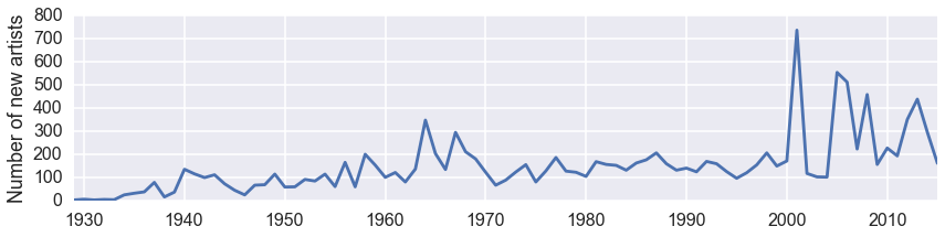
We looked above at the rate at which MOMA acquires items. Now, let’s examine the rate at which it adds artists to its collection.

We can use drop_duplicates to eliminate all but the first record with a given Artist, i.e. to remove all items except the first acquisition of an artist’s work. We save this in a new DataFrame, and group and plot it as before.

# This is a DataFrame where all items by an artist except their first acquisition are removed
firsts = moma.drop_duplicates('Artist')

fig, ax = plt.subplots(figsize=(14, 3))

(firsts.groupby(pd.Grouper(key='DateAcquired', freq='A'))
 .size()
 .plot())

ax.set_xlabel('');
ax.set_ylabel('Number of new artists');

Let’s look at trends in the acquisition of the top few artists in the collection of the Painting & Sculpture department, i.e. the people who make paintings, sculptures and installations. First we create a list of who these people are.

top = list(moma[moma['Department'] == 'Painting & Sculpture']
            .groupby('Artist')
            .size()
            .sort_values()
            .tail(8)
            .index)

Then we use the isin() method of a series to construct a boolean Series to filter out people who are not in that list.

with sns.color_palette(palette='husl', n_colors=8):  # more than 6 colors
    fig, ax = plt.subplots()

    (moma[moma['Artist'].isin(top) &
          (moma['Department'] == 'Painting & Sculpture')]
     .groupby([pd.Grouper(freq='10A', key='DateAcquired'), 'Artist'])
     .size()
     .unstack()
     .plot(ax=ax))
    
    ax.set_xlabel('')

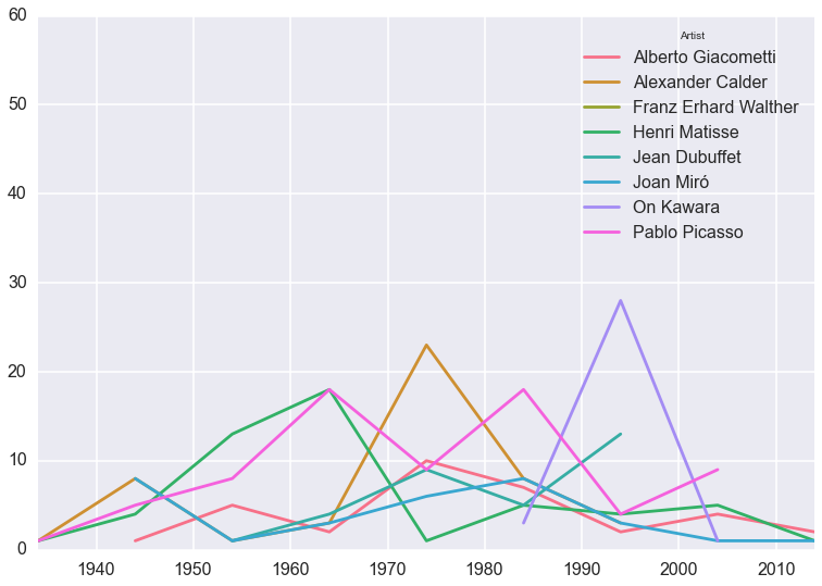
This plot is a bit of a mess, since acquisitions by such famous artists are inevitably infrequent and bursty. But clearly there were lots of Calder acquisitions in the 70s and Kawara acquisitions in the 90s.

This is the end of the first post on the MOMA collection dataset. In the second post, I’ll look at how the rate at which MOMA acquires work by women has varied over time.